ECO 2011

你或许会更想去 Notekit 看这份笔记

• Ten Principles of Economics

  • Marginal Change: A small incremental adjustment to an existing plan of action.

  • Prices:

    • Determined by interaction of buyers and sellers

    • Reflect the good’s value to society

    • Reflect the cost of producing the goods

  • Invisible Handby Adam Smith:

    • Prices guide self-interested households and firms to make decisions that maximize society’s economic well-being.

  • Gov: Enforce property rights.

  • Externality & Market Power -> Market Failure

  • The Circular-Flow Diagram

    Figure
    

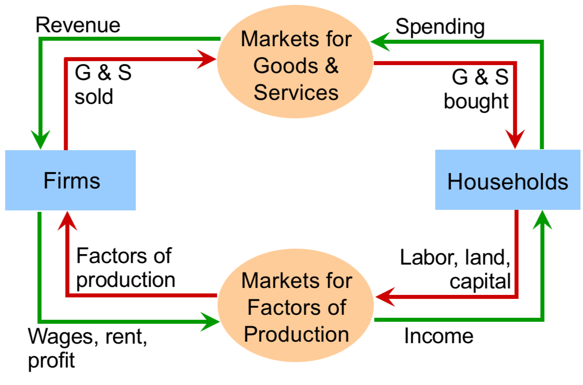
    A visual model of the economy, shows how dollars flow through markets among households and firms

    Two types of “actors”
    Households
    Own the factors of production, sell/rent them to firms for income

    Buy and consume goods& services

    Firms
    Buy/hire factors of production, use them to produce goods and services

    Sell goods & services

    Include two markets
    The market for goods and services

    The market for “factors of production”

  • Positive and Normative Statement

    • Positive Statement: 描述现在是什么, 可以被证伪（Evaluated by analyzing data; Can be Confirmed or Refuted）

    • Normative Statement: 描述将来怎么样, 不可以被证伪（Evaluated using data, value judgments, views on ethics, region, political）

• The Production Possibilities Frontier

  • PPF Example

    （*现在同样的资源, 可造5000小麦或者500电脑, 电脑难造小麦容易造）

    当这条线越靠近Y轴, 斜率越大时（比如X轴截距100, 说明现在的资源可造5000小麦或100电脑）, 说明X轴表示的东西变得更难获得、Y轴表示的东西变得更容易获得, X轴的Opportunity Cost变大, Y轴的Opportunity Cost变小

    当这条线越靠近X轴, 斜率越小时（比如X轴截距600, 说明现在的资源可造5000小麦或600电脑）, 说明X轴表示的东西变得容易获得、Y轴表示的东西变得更难获得, X轴的Opportunity Cost变小, Y轴的Opportunity Cost变大

    总结
    靠近哪个轴这哪个轴东西容易获得, Oppurtunity Cost小 例

    斜率代表的是X轴所代表物品的Opportunity Cost

    PPF becomes steeper and the opportunity cost of mountain bikes increases

  • 表述：The opportunity cost of A in terms of B

  • Outward是凸的, Inward是凹的, Feasible是可以达到的

  • Usually bentoutward: due to the law of increasing opportunity cost

    • Resources suited to computer production are used in the car industry.

    • Technological advance in producing one thing: Move one endpoint while another stays the same.

  • Points under PPF: Not efficient(widespread unemployment); Points above PPF: Not feasible.

• Comparative Advantage (-> Specialization)

  • Abs advantage: Produce with fewer inputs (can have in both goods)

  • Have lower opportunity cost than another producer (impossible to have in both goods)$$Opportunity\ Cost\ of\ A=\frac{1}{Opportunity\ Cost\ of\ B}$$

  • The Price of the Trade: Must lie between their opportunity costs.

  • Comparative Advantage -> Exports; Else Imports

  • International trade can make some individuals worse off, even as it makes the country as a whole better off; Same comparative advantage -> No gains

• Demand & Supply

  • Demand:

    • Price Up; Quantity Down

    • Shift:

      • Increase -> Right; Decrease -> Left

      • Shifters:

        • Income

          • Normal Goods:((An increase in income leads to an increase in demand))

          • Inferior Goods:((An increase in income leads to a decrease in demand))

        • Prices of Related Goods

          • Substitutes: A’s price Up, A’s demand Down; B’s demand Up

          • Complements: A’s Price Up, A’s demand Down; B’s demand Down

        • Tastes

        • Expectations

          • Expect income Up; Current demand Up

          • Expect price Up; Current demand Up

        • Number of Buyers

      • Price of the good itself -> a movement along the demand curve

  • Supply:

    • Price Up; Quantity Up

    • Shift:

      • Increase -> Right; Decrease -> Left

      • Shifters:

        • Input Prices: Input price Up; The supply Down

        • Technology: Advance in Technology, Cost Down; Supply Up

        • Expectations: Expect Price Up in the future, Supply Down Today (put some of its current production into storage)

        • Number of Sellers

      • Price of the good itself represents a movement along the curve

  • Equilibrium Price (Marketing-clearing Price)

    • Surplus:$$Q_S > Q_D$$Price Down

    • Shortage:$$Q_D>Q_S$$Price Up

• Elasticity

  • Price Elasticity of Demand

    • How much the$$Q^d$$responds to a change in price

    • If we say it is free to enter/leave the market, elasticity ishigh.

    • Determinants

      • Avaiability of Close Substitutes: With close substitutes -> High Elasticity

      • Necessities -> Inelastic; Luxuries -> Elastic

      • Definition Narrow -> Elastic; Broad -> Inelastic

      • Longer time horizons -> Elastic

    • $$Price\ Elasticity\ of\ Demand = \frac{ \%\ change\ in\ Q_D}{\%\ change\ in\ Price}=\frac{\frac{Q_2-Q_1}{\frac{1}{2}(Q_2+Q_1)}}{\frac{P_2-P_1}{\frac{1}{2}(P_2+P_1)}} = \frac{(Q_2-Q_1)(P_2+P_1)}{(Q_2+Q_1)(P_2-P_1)}=\frac{P}{Q} \times \frac{1}{\frac{\Delta P}{\Delta Q} } = \frac{P}{Q} \times \frac{1}{k}$$

      • Whenkis a constant, (P up Q down) -> Elasticity Up.

        • 

      • AlwaysPOSITIVE

    • Variety: Elastic(>1); Unit Elastic(=1); Inelastic(<1)

    • 注：想象Inelastic的I是竖直的, 所以竖线是Perfect Inelastic, Elasticity为0. 故斜率越大越Inelastic, 斜率越小越Elastic, 为0是横线Perfect Elastic, Elasticity为无穷

    • Total Revenue and the Price Elasticity of Demand

      • Inelastic: Price Up, Revenue Up; Elastic: Price Up, Revenue Down; Unit Elastic: Price Change, Total Revenue Remains Constant

  • The Income Elasticity of Demand

    • $$Income\ Elasticity\ of\ Demand = \frac{ \%\ change\ in\ Q_D}{\%\ change\ in\ Income}$$

    • Normal Goods: Positive

      • Necessities: Small

      • Luxuries: Large

    • Inferior Goods: Negative

  • The Cross-Price Elasticity of Demand

    • $$CrossPrice\ Elasticity\ of\ Demand = \frac{\%\ change\ Q_D\ of\ A}{\%\ change\ P\ of\ B}$$

    • Substitutes: Positive; Complements: Negative

  • The Price Elasticity of Supply

    • Determinants: The flexibility of sellers to change the amount of the good they produce (Easy to change, Elasticity Up)

    • More elastic in the long run than short

    • $$Price\ Elasticity\ of\ Supply=\frac{\%\ change\ in\ Q_S}{\%\ change\ in\ P}$$

• Consumer and Producer Surplus

  • Consumer Surplus

    • $$CS=WTP-P\ (*Always\ \ge 0)$$

    • The area below D-curve and above the Price.

    • Lower Price -> Additional consumer surplus to initial consumers + Consumer surplus to new consumers

  • Producer Surplus

    • $$PS=P-Cost$$

      • Cost: The value of everything a seller must give up to produce a good. *Lowest price / Producer’s willingess to sell his services

    • The area below the Price and above the S-curve.

    • Higher Price -> Additional producer surplus to initial producers + Producer surplus to new producers

  • Market Efficiency

    • $$Total\ Surplus=Consumer\ Surplus+Producer\ Surplus=Value\ to\ Buyers-Cost\ to\ Sellers$$

    • Efficiency -> Maximize Total Surplus received by all members

    • Equality -> Distributing Economic Prosperity Uniformly Among the members of Society

• Government Intervention

  • Price ceiling / Price floor

    • Binding 才是有效的, 即 Ceiling 高需低于 Eq’m Price 方为 Binding, Floor 需高于 Eq’m Price

    • DWL: Triangle Area

    • Labor Market: Price Floor means minimum wage. So minimum wage causes a labor surplus(unemployment).

    • Price ceiling -> Shortage. In the long run, supply and demand are more price-elastic. Shortage is larger.

      • -> Sellers must ration the goods among the buyers.

        • Long lines; Discrimination according to sellers’ biases -> Often unfair and inefficient (goods do not go to buyers who value the goods most)

    • Apartment Rent, in the short run, we haveperfect inelastic supply.

  • Taxes

    • 

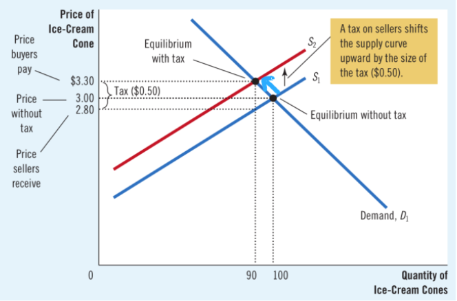
    • Discourage Market Activity. Eq’m Quantity Down.

    • $$Tax\ Revenue=Tax \times New\ Eq’m\ Quantity$$

    • DWL: The fall in total surplus that results from a market distortion. Triangle Area.

    • Elasticity & Tax Burden

      • Buyers/Sellers who havelower elasticitywill have alarger tax burden. A tax burden falls more heavily on the side of the market that is less elastic. Because fewer good alternatives and less willing to leave the market.

    • Thegreatertheelasticitiesof supply and demand, thelargerthedeadweight losscaused by the tax.

  • The Determinants of Trade

    • Word Price > Domestic Price -> Export (Opp cost low)
      Word Price < Domestic Price -> Import (Opp cost high)

    • For Exporting Country:
      Domestic producers better off
      Domestic consumers worse off
      Economic well-being Up

    • For Importing Country:
      Domestic consumers better off
      Domestic producers worse off
      Economic well-being Up

    • Tariff (Works forimporter)

      • 

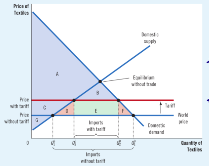
      • a tax on imported goods

      • Causes DWL(Overproduction & Underconsumption). Best policy for eficiency is to allow trade without a tariff.

  • Price Support

    • 

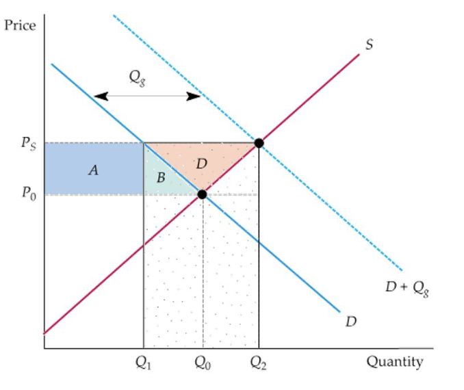
    • Price Supports

      $$\Delta Welfare=D-(Q_2-Q_1)\times P_S$$

      $$\Delta PS = A+B+D$$

      $$\Delta CS=-A-B$$

      $$Gov\ Buy=Q_2-Q_1$$

      $$Gov\ Cost= (Q_2-Q_1)\times P_S $$

  • Production Quotas

    • 

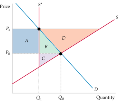
    • $$\Delta Welfare=-(B+C)$$

  • Incentive Program

    • 

    • $$Min\ Incentive=B+C+D\ \Delta CS=-(A+B)\ \Delta PS=(A+B+D)\ \Delta Welfare=-(B+C)$$

• Externality

  • Gov correct byinternalize the externality

    • Negative Externalities:$$Q^* < Q_{Market}$$, Tax

    • Positive Externalities:$$Q^* > Q_{Market}$$, Subsidize

  • Public Policies towards Externalities

    • Command-and-Control Policies: Regulation (Req/Forbid)

    • Market-based Policy: Corrective Taxes (Pigouvian Taxes) & Subsidies

      • $$Ideal\ Corrective\ Tax/Subsidy = External\ Cost/Benefit$$

      • Rather than causing DWL, actually makes the economy work better

    • Tradable Pollution Permits

      • Corrective Tax: Sets the price of pollution; Pollution: Perfectly elastic

      • Pollution Permits: Sets the quantity of pollution; Pollution: Perfectly inelastic

  • Private Solutions to Externalities

    • Moral Codes & Social Sanctions
      Charities
      Merge/Contract

    • The Coase Theorem

      • Bargain without cost over the allocation of resources -> Solve the problem of externalities on their own

      • Do NOT Work when

        • Transaction Costs are high.

        • A beneficial aggrement exists. Each party may hold out for a better deal.

        • The number of interested parties is large -> reaching efficient is difficult.

• Public Goods and Common Resources

  • Excludability: 一个人是否可以被阻止使用

  • Rivalry in consumption: 一个人用是否使他人使用减少

  • 四种分类（Congested: Rival; Toll: Excludable）

        - Rival

        - Not Rival

    - Excludable

        - Private Goods

            - Congested Toll Roads

        - Club Goods

            - Uncongested Toll Roads

    - Not Excludable

        - Common Resources

            - Congested Nontoll Roads

        - Public Goods

            - Uncongested Nontoll Roads

- ((Public Goods))underprovided

    - The Free-Rider Problem

    - e.g. National Defense; Basic Research(General Knowledge)

    - Cost-benefit analyses are imprecise (Fair cost-sharing & Truthful Reporting)

- ((Common Resources))overconsumed

    - The Tragedy of the Commons: People neglect the external cost -> overuse

    - e.g. Clean Air and Water; Fish, Whales and Other Wildlife

    - Regulate; Corrective Tax; Permits; Convert to private

• Consumer Theory

  • The Budget Constraint

    • Limit on the consumption (bundles/combination) a consumer can afford

    • Slope:$$Relative\ Price=\frac{P_x}{P_y}$$

    • $$P_x\ x + P_y \ y=I$$

  • Indifference Curves

    • Bundles giving the consumer the same level of satisfaction.

    • Slope:$$MRS=\frac{MU_x}{MU_y}$$(Marginal Rate of Substitution)

      • 他想要用几个Y轴商品换一个X轴商品, 越大说明不想要Y想要X, 越小说明不想要X想要Y.

      • Example: 在此点由于斜率是大的, 说明MRS是大的. 此时我有少少的x, $$MU_x$$大, 多多的y, $$MU_y$$小. 此时$$MRS=\frac{MU_x}{MU_y}$$是大的.

    • Assumptions:

      • Completeness: Consumers can compare and rank all possible baskets

      • Transitivity: Preferences are transitive.

      • More is better than less: Higher indifference curves are preferred to lower ones.

      • -> Properties

        • Higher is better.

        • Slope downward.

        • Do not cross.

        • Bowed inward.

    • Types:

      • Perfect Substitutes: MRS fixed, Straight lines

      • Close substitutes: not very bowed

      • Perfect Complements: MRS 0/Inf, L-shaped, right-angle

      • Close complements: very bowed

  • Utility

    • Score of satisfaction

    • Utility Function: a set of indiference curves each with anumerical indicator$$U(x,y)=2x+y \Rightarrow MU_x=2,\ MU_y=1$$

    • Marginal Utility(MU): Additioinal satisfaction from 1 additional unit of a good

      • Diminishing Marginal Utility: More consumed, less additions to utility from additional amounts

    • At the optimum:$$\frac{MU_x}{P_x} =\frac{MU_y}{P_y}$$

      • If$$\frac{MU_x}{P_x} \gt \frac{MU_y}{P_y}$$, that means the marginal utility from an additional unit of x is larger than that of y, so we spend more on x. As we haveDiminishing Marginal Utility,$$\frac{MU_x}{P_x} \downarrow$$, finally they equal and we are at the optimum.

      • So$$MRS=\frac{MU_x}{MU_y}=Relative\ Price=\frac{P_x}{P_y}$$

• Production Theory

  • Factors

    • Production Technology

    • Cost Constraints

    • Input Choices

  • Prod Func: highest output that a firm can produce for every specified combination of inputs$$q=f(K,L)$$

  • Production with Labor Variable

    • $$Marginal\ Product \gt Average\ Product \Rightarrow AP \uparrow\ MP=AP \Rightarrow AP_{max}\MP=0 \Rightarrow TP_{max}$$

    • Law of Diminishing Marginal Returns

      • Assume that all labor inputs are of equal quality

  • Production with Two Variable Inputs

    • Isoquants

      • All possible combinations of inputs to yield the same output. 我们总是把x轴为劳动力, y轴为资本

      • 

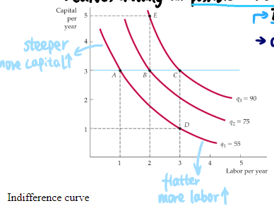
      • $$A \rightarrow B \rightarrow C \Rightarrow Diminishing\ Marginal\ Returns\ to\ Labor$$第一次增加1劳动力多生产20, 第二次增加1劳动力只多生产15

      • $$D \rightarrow B \rightarrow E \Rightarrow Diminishing\ Marginal\ Returns\ to\ Capital$$第一次多增加1资本多生产20, 第二次15

      • Slope: Marginal Rate of Technical Substitution$$MRTS=\frac{MP_L}{MP_K}=-\frac{\Delta K}{\Delta L}$$

        • 几个Capital能顶得上1个Labor

      • Downward sloping and convex

      • Special Cases

        • Perfect Substitutes: Straight Lines; MRTS Constant

        • Fixed-proportions Production Function: L-shaped; One labor - One capital

      • Returns to Scale

        • 

    • Isocosts

      • Cost

        • $$TC=Explicit+Implicit\ Cost=FC+VC\Econ\ Profit=TR-TC\Acct\ Profit=TR-Explicit\ Cost$$

      • Marginal Cost:$$\uparrow Total\ Cost\ from\ 1\ extra\ unit\ Prod\MC=\frac{\Delta TC}{\Delta Q}$$

      • Marginal Cost corsses AVC and ATC at their minimum points.

      • 

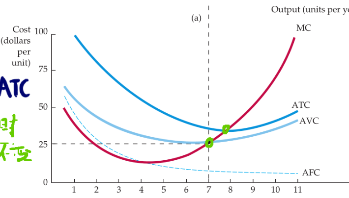
      • Sunk Cost: Expenditure that has been made and cannot be recovered. 不同于Fixed Cost, 不参与重大决策

      • Cost in the

        • Short Run: Some inputs are fixed.

          • The determinants of Short-Run Cost

            • $$MC=\frac{\Delta VC}{\Delta Q}=\frac{w\Delta L}{\Delta Q}=\frac{w}{\frac{\Delta Q}{\Delta L}}=\frac{w}{MP_L}$$So$$MP_L \uparrow\ \Rightarrow MC \downarrow $$

            • $$Quantity\ of\ Labor \uparrow\ \Rightarrow MP_L \downarrow\ \Rightarrow\ MC\uparrow$$

        • Long Run: All inputs are variable.

          • $$User\ Cost\ of\ Capital=Economic\ Depreciation + (Interest\ Rate)\times(Value\ of\ Capital)$$

          • Rate(Per dollar of capital) = Depreciation rate + Interest Rate

          • Under competitive capital market: Rent rate = User cost = Price *Rate

      • Isocost Line

        • $$C=wL+rK\K=\frac{C}{r}-\frac{w}{r}L$$

        • Optimum:$$MRTS=-\frac{\Delta K}{\Delta L}=\frac{MP_L}{MP_K}=\frac{w}{r}$$

        • If$$\frac{MP_L}{w} \gt \frac{MP_K}{r}$$, the firm will increase the use of labor and decrease the use of capital.$$Quantity\ of\ Labor \uparrow\ \Rightarrow MP_L \downarrow$$Finally we get to the optimum.

• Competitive Market

  • Assumption: Perfectly Competitive Market

    • Market with many buyers and sellers.

    • All the products are identical.

    • Firms can freely enter or exit the market.

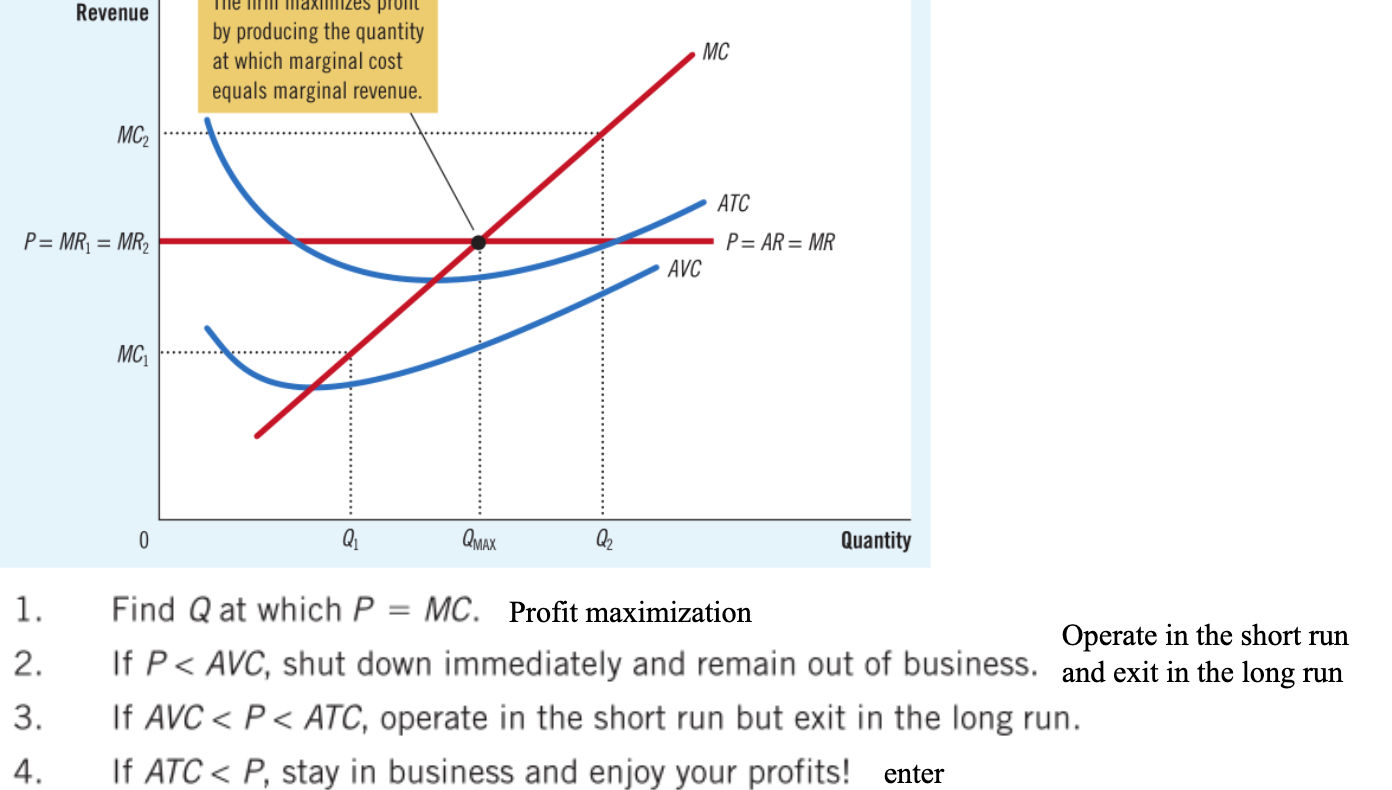
  • -> For competitive firms,$$AR=MR=P$$

  • $$TR=PQ\AR=\frac{TR}{Q}\MR=\frac{\Delta TR}{\Delta Q}\Profit_{max}\ when\ MR=MC$$

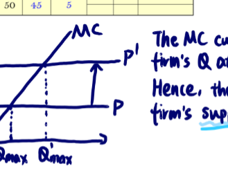
  • MC determines Q at any price. The competitive firm’sShort-Run Supply Curveis the portion of itsMC Curvethat lies above theAVC Curve.

    • 

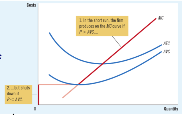    • The firm choose to shut down if$$TR<VC\ \ P<AVC$$

      • After shutting down, still need to pay fixed cost.

      • In the short run, FC are sunk costs, thus FC should not matter in the short-run decision.

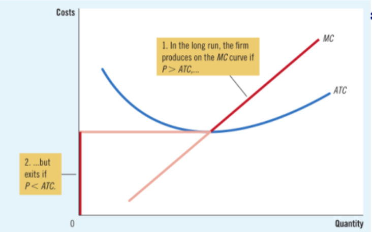
  • The competitive firm’sLong-Run Supply Curveis the portion of itsMC Curvethat lies above theATC Curve.

    • 

    • Long-Run Decision to Exit or Enter a Market

      • The firm choose to exit if$$TR<TC\ \ P<ATC$$to enter if$$TR>TC\ \ P>ATC$$

        • After exit, 0 cost.

      • $$Profit=TR-TC=(P-ATC)\times Q$$

  • Firm

  • The Supply Curve in a Competitive Market

    • The Short-Run: With a Fixed Number of Firms (Usually upward-sloping line)

    • The Long-Run: Market Supply with Entry and Exit

      • 因为有profit时就会有enter, supply增加price降低profit下降
        有loss时就会有exit, supply减少price升高profit增加

      • $$Price=Marginal\ Cost=Average\ Total\ Cost$$

      • At the minimum of ATC

  • Why Zero Profit?

    • Profit includes all includes all implicit costs. So when econ profit is zero, acct profit is positive.

  • Why Long-Run Supply Curve Might Slope Upward?

    • Horizontal: All firms have identical costs, and costs do not change as other firms enter or exit the market.

    • Upward: Firms have diferent costs, or cost rise as firms enter the market.

      • The price in the market reflects the average total cost of the marginal firm.

• Monopoly

  • Types

    • Monopoly Resources

    • Government Regulation

    • Natural Monopolies

  • Increasing Q ->

    • Higher output raises revenue

    • Lower price reduces revenue

  • To sell a larger Q, the monopolist must reduce the price on all the units it sells. => Marginal revenue is less than the price of its good.

  • MR can be negative. Price effect on revenue outweighs the output effect.

  • $$Profit\ Maximization\ P>MR=MC\ For\ a\ competitive\ firm:\ P=MR=MC$$

  • 

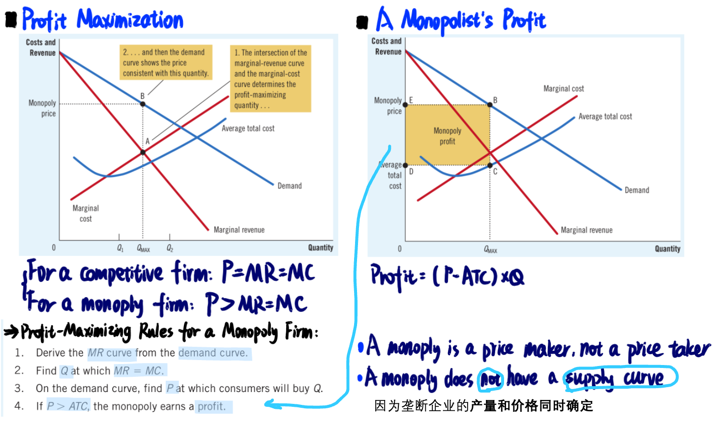
  • 在”Monopoly quantity” 右侧的某一单位产量, 消费者愿意支付的价格高于企业生产该单位的成本, 但这一单位产量没有被生产出来, 这就造成了社会福利的损失, 累积起来就是图中的红色阴影部分.

  • Price Regulation

  • The Effect of Tax

  • $$MR=\frac{\Delta R}{\Delta Q}=\frac{\Delta (PQ)}{\Delta Q}=P+Q \frac{\Delta P}{\Delta Q}=P+P(\frac{Q}{P})(\frac{\Delta P}{\Delta Q})=P+P(\frac{1}{E_d})=MC$$

  • $$P=\frac{MC}{1+\frac{1}{E_d}}$$

  • $$Markup=Lerner\ Index=\frac{P-MC}{P}=-\frac{1}{E_d}$$